Pytorch（1）张量操作

发表于 2022-04-27 更新于 2023-04-18 分类于【draft】工程，开源工具， Pytorch框架阅读次数：本文字数： 4.9k 阅读时长 ≈ 9 分钟

PyTorch 资料

PyTorch 1.7.0 文档
https://www.w3cschool.cn/pytorch/pytorch-mrni3btn.html
https://handbook.pytorch.wiki/chapter1/1.1-pytorch-introduction.html
LSTM细节分析理解（pytorch版）：https://zhuanlan.zhihu.com/p/79064602
OLD：https://www.pytorch123.com/SixthSection/Dcgan/
PyTorch 学习笔记汇总（完结撒花） - 张贤同学的文章 - 知乎 https://zhuanlan.zhihu.com/p/265394674

PyTorch 学习笔记

在线电子书：https://pytorch.zhangxiann.com/

配套代码：https://github.com/zhangxiann/PyTorch_Practice

一、基本概念

1.1 Pytorch 简介与安装

1.2 Tensor 张量介绍

1.2.1 直接创建 Tensor

torch.tensor()

1	torch.tensor(data, dtype=None, device=None, requires_grad=False, pin_memory=False)

data: 数据，可以是 list，numpy
dtype: 数据类型，默认与 data 的一致
device: 所在设备，cuda/cpu
requires_grad: 是否需要梯度
pin_memory: 是否存于锁页内存

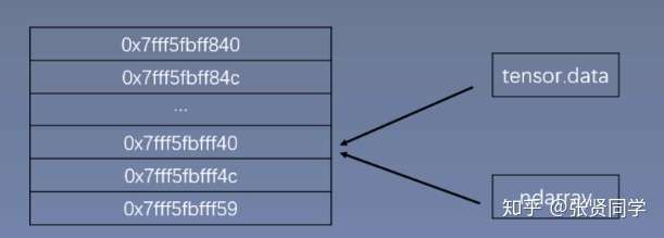
torch.from_numpy(ndarray)

从 numpy 创建 tensor。利用这个方法创建的 tensor 和原来的 ndarray 共享内存，当修改其中一个数据，另外一个也会被改动。

1.2.2 根据数值创建 Tensor

torch.zeros()：根据 size 创建全 0 张量

1	torch.zeros(*size, out=None, dtype=None, layout=torch.strided, device=None, requires_grad=False)

size: 张量的形状
out: 输出的张量，如果指定了 out，那么torch.zeros()返回的张量和 out 指向的是同一个地址
layout: 内存中布局形式，有 strided，sparse_coo 等。当是稀疏矩阵时，设置为 sparse_coo 可以减少内存占用。
device: 所在设备，cuda/cpu
requires_grad: 是否需要梯度

torch.full()，torch.full_like()：创建自定义数值的张量

1	torch.full(size, fill_value, out=None, dtype=None, layout=torch.strided, device=None, requires_grad=False)

size: 张量的形状，如 (3,3)
fill_value: 张量中每一个元素的值

torch.arange()：创建等差的 1 维张量。注意区间为[start, end)。

1	torch.arange(start=0, end, step=1, out=None, dtype=None, layout=torch.strided, device=None, requires_grad=False)

start: 数列起始值
end: 数列结束值，开区间，取不到结束值
step: 数列公差，默认为 1

torch.linspace()：创建均分的 1 维张量。数值区间为 [start, end]

1	torch.linspace(start, end, steps=100, out=None, dtype=None, layout=torch.strided, device=None, requires_grad=False)

start: 数列起始值
end: 数列结束值
steps: 数列长度 (元素个数)

1.2.3 根据概率创建 Tensor

torch.normal()

1	torch.normal(mean, std, *, generator=None, out=None)

功能：生成正态分布 (高斯分布)

mean: 均值
std: 标准差

==1.3 张量操作与线性回归==

==1.3.1 拼接==：cat、stack

torch.cat()：将张量按照 dim 维度进行拼接

1	torch.cat(tensors, dim=0, out=None)

tensors: 张量序列 [t, t]
dim: 要拼接的维度

torch.stack()：将张量在==新创建的 dim 维度==上进行拼接，已有维度后移

1	torch.stack(tensors, dim=0, out=None)

tensors: 张量序列
dim: 要拼接的维度

==1.3.2 切分==：chunk、split

torch.chunk()：将张量按照维度 dim 进行平均切分。若不能整除，则最后一份张量小于其他张量。

1 2	torch.chunk(input, chunks, dim=0) torch.chunk(a, dim=1, chunks=3)

input: 要切分的张量
chunks: 要切分的份数
dim: 要切分的维度

torch.split()：将张量按照维度 dim 进行平均切分。可以指定每一个==分量的切分长度==。

1 2	torch.split(tensor, split_size_or_sections, dim=0) torch.split(t, [2, 1, 2], dim=1)

tensor: 要切分的张量
split_size_or_sections: 为 int 时，表示每一份的长度，如果不能被整除，则最后一份张量小于其他张量；为 list 时，按照 list 元素作为每一个分量的长度切分。如果 list 元素之和不等于切分维度 (dim) 的值，就会报错。
dim: 要切分的维度

==1.3.3 索引==

torch.index_select()：在维度 dim 上，按照 index 索引取出数据拼接为张量返回。

1	torch.index_select(input, dim, index, out=None)

功能：在维度 dim 上，按照 index 索引取出数据拼接为张量返回。torch.tensor([0, 2], dtype=torch.long)

input: 要索引的张量
dim: 要索引的维度
index: 要索引数据的序号

torch.mask_select()：按照 mask 中的 True 进行索引拼接得到一维张量返回。

1	torch.masked_select(input, mask, out=None)

要索引的张量
mask: 与 input 同形状的布尔类型张量

==1.3.4 变换==

torch.reshape()：变换张量的形状。当张量在内存中是连续时，返回的张量和原来的张量共享数据内存，改变一个变量时，另一个变量也会被改变。

1 2	torch.reshape(input, shape) torch.reshape(t, (-1, 2, 2))

input: 要变换的张量
shape: 新张量的形状

torch.transpose()：交换张量的两个维度。常用于图像的变换，比如把`chw`变换为`hwc`。

1	torch.transpose(input, dim0, dim1)

input: 要交换的变量
dim0: 要交换的第一个维度
dim1: 要交换的第二个维度

torch.t()：2 维张量转置，对于 2 维矩阵而言，等价于`torch.transpose(input, 0, 1)`。

torch.squeeze()：压缩长度为 1 的维度

1	torch.squeeze(input, dim=None, out=None)

dim: 若为 None，则移除所有长度为 1 的维度；若指定维度，则当且仅当该维度长度为 1 时可以移除。

torch.unsqueeze()：根据 dim 扩展维度，长度为 1。

1	torch.unsqueeze(input, dim)

==1.3.5 张量的数学运算==

加减乘除，对数，指数，幂函数和三角函数。

torch.add(): 逐元素计算 input + alpha * other。因为在深度学习中经常用到先乘后加的操作。

1 2	torch.add(input, other, out=None) torch.add(input, other, *, alpha=1, out=None)

input: 第一个张量
alpha: 乘项因子
other: 第二个张量

torch.addcdiv()

1	torch.addcdiv(input, tensor1, tensor2, *, value=1, out=None)

计算公式为：out $_{i}=\operatorname{input}_{i}+$ value $\times \frac{\text { tensor } 1_{i}}{\text { tensor } 2_{i}}$

torch.addcmul()

1	torch.addcmul(input, tensor1, tensor2, *, value=1, out=None)

计算公式为：out $_{i}=$ input $_{i}+$ value $\times$ tensor $1_{i} \times$ tensor $2_{i}$

==Pytorch 线性回归==

线性回归是分析一个变量 ( $y$ ) 与另外一 (多) 个变量 ( $x$ ) 之间的关系的方法。一般可以写成 $y=wx+b$ 。线性回归的目的就是求解参数 $w, b$ 。

线性回归的求解可以分为 3 步：

确定模型： $y=wx+b$
选择损失函数，一般使用均方误差 MSE： $\frac{1}{m} \sum_{i=1}^{m}\left(y_{i}-\hat{y}_{i}\right)^{2}$ 。其中 $\hat{y}_{i}$ 是预测值， $y$ 是真实值。
使用梯度下降法求解梯度 (其中 $lr$ 是学习率)，并更新参数：

$w = w - lr * w.grad$
$b = b - lr * b.grad$

代码如下：

import torch
import matplotlib.pyplot as plt
torch.manual_seed(10)

lr = 0.05  # 学习率

# 创建训练数据
x = torch.rand(20, 1) * 10  # x data (tensor), shape=(20, 1)
# torch.randn(20, 1) 用于添加噪声
y = 2*x + (5 + torch.randn(20, 1))  # y data (tensor), shape=(20, 1)

# 构建线性回归参数
w = torch.randn((1), requires_grad=True) # 设置梯度求解为 true
b = torch.zeros((1), requires_grad=True) # 设置梯度求解为 true

# 迭代训练 1000 次
for iteration in range(1000):

    # 前向传播，计算预测值
    wx = torch.mul(w, x)
    y_pred = torch.add(wx, b)

    # 计算 MSE loss
    loss = (0.5 * (y - y_pred) ** 2).mean()

    # 反向传播
    loss.backward()

    # 更新参数
    b.data.sub_(lr * b.grad)
    w.data.sub_(lr * w.grad)

    # 每次更新参数之后，都要清零张量的梯度
    w.grad.zero_()
    b.grad.zero_()

    # 绘图，每隔 20 次重新绘制直线
    if iteration % 20 == 0:

        plt.scatter(x.data.numpy(), y.data.numpy())
        plt.plot(x.data.numpy(), y_pred.data.numpy(), 'r-', lw=5)
        plt.text(2, 20, 'Loss=%.4f' % loss.data.numpy(), fontdict={'size': 20, 'color':  'red'})
        plt.xlim(1.5, 10)
        plt.ylim(8, 28)
        plt.title("Iteration: {}\nw: {} b: {}".format(iteration, w.data.numpy(), b.data.numpy()))
        plt.pause(0.5)

        # 如果 MSE 小于 1，则停止训练
        if loss.data.numpy() < 1:
            break